
PUMPA - SMART LEARNING
எங்கள் ஆசிரியர்களுடன் 1-ஆன்-1 ஆலோசனை நேரத்தைப் பெறுங்கள். டாப்பர் ஆவதற்கு நாங்கள் பயிற்சி அளிப்போம்
Book Free DemoWe will see a few cases which can elaborate on the relation between time and distance.

The above figure shows a bike travelling along a straight line away from the starting point O with uniform speed.
The distance of the bike is measured for every second. The distance and time are recorded, and a graph is plotted using the data. The below graph shows the possible results of the journey.
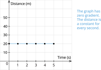
Case I: If the bike staying at rest, then the distance is constant for every second.
| Time(s) | 0 | 1 | 2 | 3 | 4 | 5 |
| Distances(m) | 0 | 20 | 20 | 20 | 20 | 20 |
If we plot a graph for the constant distance, we get a straight line, as shown in the below graph.
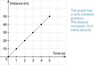
Case II: The bike travelling at a uniform speed of 10 \frac{m}{s}
| Time(s) | 0 | 1 | 2 | 3 | 4 | 5 |
| Distances(m) | 0 | 10 | 20 | 30 | 40 | 50 |
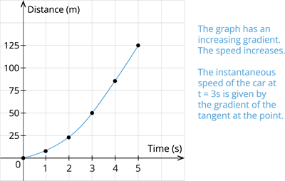
Case III: The bike travelling at increasing speed.
| Time(s) | 0 | 1 | 2 | 3 | 4 | 5 |
| Distances(m) | 0 | 5 | 20 | 45 | 80 | 125 |
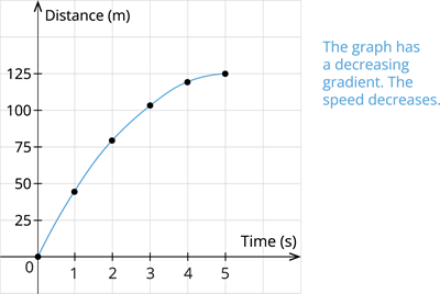
Case IV: The bike travelling at decreasing speed.
| Time(s) | 0 | 1 | 2 | 3 | 4 | 5 |
| Distances(m) | 0 | 45 | 80 | 105 | 120 | 125 |
 Register for free to see more content